
Notice
Recent Posts
Recent Comments
Link
| 일 | 월 | 화 | 수 | 목 | 금 | 토 |
|---|---|---|---|---|---|---|
| 1 | 2 | 3 | ||||
| 4 | 5 | 6 | 7 | 8 | 9 | 10 |
| 11 | 12 | 13 | 14 | 15 | 16 | 17 |
| 18 | 19 | 20 | 21 | 22 | 23 | 24 |
| 25 | 26 | 27 | 28 | 29 | 30 | 31 |
Tags
- 유럽 교환학생
- 미래에셋해외교환
- m1 anaconda 설치
- special method
- 특별 메소드
- 유럽
- Deeplearning
- fluent python
- anaconda 가상환경
- 미래에셋 장학생
- set add
- 선형회귀
- Python
- li-ion
- Machine learning
- gradient descent
- 2022년
- 오스트리아
- cost function
- 양극재
- 나의23살
- electrochemical models
- Andrew ng
- 딥러닝
- 청춘 화이팅
- set method
- fatigue fracture
- 이차전지
- 교환학생
- Linear Regression
Archives
- Today
- Total
Done is Better Than Perfect
[딥러닝] 3. 딥러닝 모델 구현 (선형 회귀, 비선형 회귀 모델 구현) 본문
' 딥러닝 모델 구현 순서' 는 다음과 같다.
1. 데이터셋 준비하기
2. 딥러닝 모델 구축하기
3. 모델 학습 시키기
4. 평가 및 예측하기
아래에서는 각 단계에서 필요한 개념을 쭉 훌어본 후에, tensorflow 코드로 선형 회귀와 비선형 회귀를 구현해보겠다.
1. 데이터셋 준비하기
- epoch : 한 번의 epoch는 전체 데이터 셋에 대해 한 번 학습을 완료한 상태
- batch : 나눠진 데이터셋 (보통 mini-batch라 표현)
- iteration는 epoch를 나누어서 실행하는 횟수를 의미함

2. 딥러닝 모델 구축하기
[ keras 예시 코드 - 아래 두개는 동일한 코드임 ]
model = tf.keras.models.Sequential([
	tf.keras.layers.Dense(10,input_dim=2, activation='sigmoid'),
    tf.keras.layers.Dense(10, activation='sigmoid'),
    tf.keras.layers.Dense(1, activation='sigmoid')
    ])
model = tf.keras.models.Sequential()
model.add(tf.keras.layers.Dense(10,input_dim=2, activation='sigmoid'))
model.add(tf.keras.layers.Dense(10, activation='sigmoid'))
model.add(tf.keras.layers.Dense(1, activation='sigmoid'))
3. 모델 학습 시키기
[model].compile(optimizer, loss) : 모델의 학습을 설정하기 위한 함수
- optimizer : 모델 학습 최적화 방법
- loss : 손실 함수 설정
[model].fit(x,y) : 모델을 학습시키기 위한 함수
- x : 학습 데이터
- y : 학습 데이터의 label
[ 예시 코드 ]
model.compile(loss='mean_squared_error', optimizer='SGD')
model.fit(dataset, epochs=100)
4. 평가 및 예측하기
[model].evaluate(x,y) : 모델을 평가하기 위한 함수
- x : 테스트 데이터
- y : 테스트 데이터의 label
[model].predict(x) : 모델로 예측을 수행하기 위한 함수
- x : 예측하고자 하는 데이터
[ 예시 코드 ]
# 테스트 데이터 준비하기
dataset_test = tf.data.Dataset.from_tensor_slices((data_test, labels_test))
dataset_test = dataset.batch(32)

# 모델 평가 및 예측하기
model.evaluate(dataset_test)
predicted_labels_test = model.predict(data_test)
딥러닝 모델 구현
tensorflow 코드로 선형 회귀와 비선형 회귀를 구현
1. 선형 회귀 모델 구현
import tensorflow as tf
import matplotlib.pyplot as plt
import matplotlib as mpl
import numpy as np
import os
np.random.seed(100)

'''
1. 선형 회귀 모델의 클래스를 구현
   Step01. 가중치 초기값을 1.5의 값을 가진 변수 텐서로 설정
   Step02. Bias 초기값을 1.5의 값을 가진 변수 텐서로 설정
   Step03. W, X, b를 사용해 선형 모델 구현
'''
class LinearModel:

    def __init__(self):
        self.W = tf.Variable(initial_value=1.5)
        self.b = tf.Variable(initial_value=1.5)

    def __call__(self, X, Y):
        return X * self.W + self.b

''' 2. MSE를 loss function으로 사용 '''
def loss(y, pred):
    return tf.reduce_mean(tf.square(y-pred))

'''
3. gradient descent 방식으로 학습하는 train 함수 정의 - W(가중치)와 b(Bias) 업데이트
'''

def train(linear_model, x, y):

    with tf.GradientTape() as t:
        current_loss = loss(y, linear_model(x, y))

    learning_rate = 0.001

    # gradient 값 계산
    delta_W, delta_b = t.gradient(current_loss, [linear_model.W, linear_model.b])

    # learning rate와 계산한 gradient 값을 이용하여 업데이트할 파라미터 변화 값 계산
    W_update = (learning_rate * delta_W)
    b_update = (learning_rate * delta_b)

    return W_update,b_update

def main():

    # 데이터 생성
    x_data = np.linspace(0, 10, 50)
    y_data = 4 * x_data + np.random.randn(*x_data.shape)*4 + 3

    # 데이터 출력
    plt.scatter(x_data,y_data)
    plt.show()

    # 선형 함수 적용
    linear_model = LinearModel()

    epochs = 100
    for epoch_count in range(epochs): # epoch 값만큼 모델 학습

        # 선형 모델의 예측 값 저장
        y_pred_data = linear_model(x_data, y_data)

        # 예측 값과 실제 데이터 값과의 loss 함수 값 저장
        real_loss = loss(y_data, linear_model(x_data, y_data))

        # 현재의 선형 모델을 사용하여  loss 값을 줄이는 새로운 파라미터로 갱신할 파라미터 변화 값 계산
        update_W, update_b = train(linear_model, x_data, y_data)

        # 선형 모델의 가중치와 Bias 업데이트
        linear_model.W.assign_sub(update_W)
        linear_model.b.assign_sub(update_b)

        if (epoch_count%20==0):
            print(f"Epoch count {epoch_count}: Loss value: {real_loss.numpy()}")
            print('W: {}, b: {}'.format(linear_model.W.numpy(), linear_model.b.numpy()))

            fig = plt.figure()
            ax1 = fig.add_subplot(111)
            ax1.scatter(x_data,y_data)
            ax1.plot(x_data,y_pred_data, color='red')
            plt.savefig('prediction.png')
            plt.show()

if __name__ == "__main__":
    main()
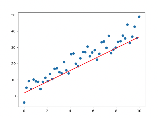
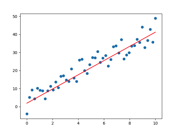
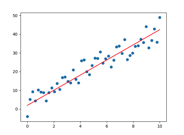
[ 코드 실행 결과 ]
- epoch 진행될 수록 loss 값이 떨어지므로, 학습이 잘 이루어지고 있음
- Weight, bias 값이 업데이트 됨
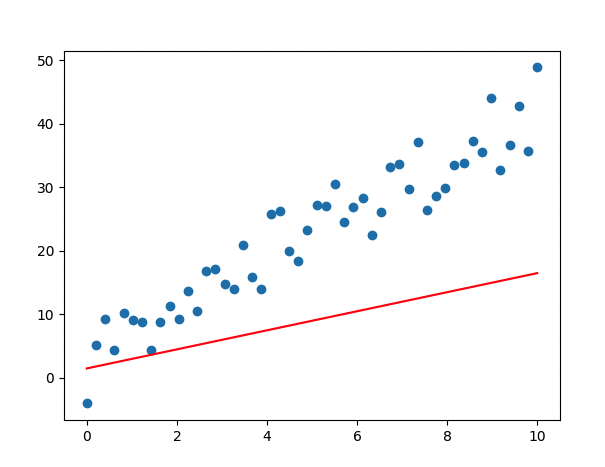
## output ##

Epoch count 0: Loss value: 250.49554443359375
W: 1.677997350692749, b: 1.527673602104187
Epoch count 20: Loss value: 28.3988094329834
W: 3.5059425830841064, b: 1.8219205141067505
Epoch count 40: Loss value: 15.571966171264648
W: 3.942619800567627, b: 1.907819151878357
Epoch count 60: Loss value: 14.813202857971191
W: 4.045225143432617, b: 1.9435327053070068
Epoch count 80: Loss value: 14.750727653503418
W: 4.067629814147949, b: 1.9670435190200806
2. 비선형 회귀 모델 구현
import tensorflow as tf
import numpy as np
from visual import *
import os
np.random.seed(100)
tf.random.set_seed(100)
def main():
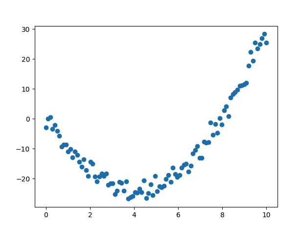
# 비선형 데이터 생성
x_data = np.linspace(0, 10, 100)
y_data = 1.5 * x_data**2 -12 * x_data + np.random.randn(*x_data.shape)*2 + 0.5
''' 1. 다층 퍼셉트론 모델 생성 '''
# units : 레이어안의 노드 수
# activation : 적용할 activation function
model = tf.keras.models.Sequential([
tf.keras.layers.Dense(units=20, input_dim=1, activation='relu'),
tf.keras.layers.Dense(units=20, activation='relu'),
tf.keras.layers.Dense(units=1)
])
''' 2. 모델 학습 방법 설정 '''
# 모델을 학습시킬 손실 함수(loss function) 계산 방법과 최적화(optimize) 방법 설정
model.compile(loss = 'mean_squared_error', optimizer = 'adam')
''' 3. 모델 학습 '''
# 생성한 모델을 500 epochs 만큼 학습시킴. verbose는 모델 학습 과정 정보를 얼마나 자세히 출력할지를 설정함
history = model.fit(x_data, y_data, epochs=500, verbose=2)
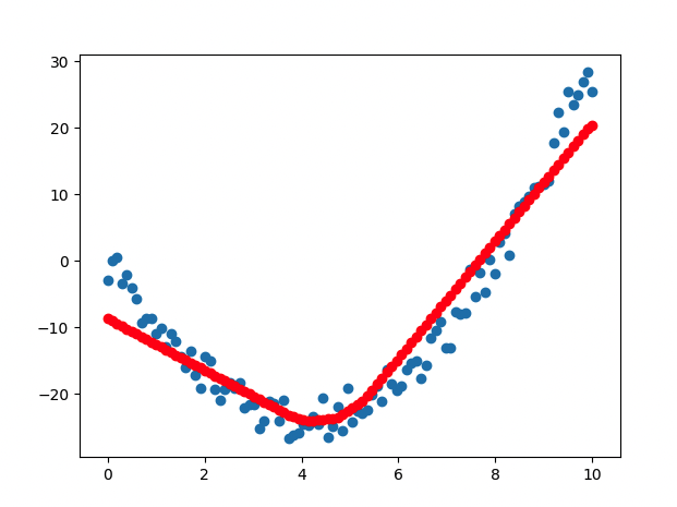
''' 4. 학습된 모델을 사용하여 예측값 생성 및 저장 '''
# 학습한 모델을 사용하여 x_data에 대한 예측값 생성
predictions = model.predict(x_data)
Visualize(x_data, y_data, predictions)
return history, model
if __name__ == '__main__':
main()
[ 코드 실행 결과 ]
- epoch 진행될 수록 loss 값이 떨어지므로, 학습이 잘 이루어지고 있음
- Weight, bias 값이 업데이트 됨
Epoch 1/500
100/100 - 0s - loss: 290.6330
Epoch 250/500
100/100 - 0s - loss: 86.8522
Epoch 500/500
100/100 - 0s - loss: 15.2892
'🤖 AI > Deep Learning' 카테고리의 다른 글
| [딥러닝] 6. 딥러닝 모델 학습의 문제점 pt.3 : 과적합 (0) | 2024.06.22 |
|---|---|
| [딥러닝] 5. 딥러닝 모델 학습의 문제점 pt.2 : 기울기 소실, 가중치 초기화 방법 (2) | 2024.06.12 |
| [딥러닝] 4. 딥러닝 모델 학습의 문제점 pt.1 : 최적화 알고리즘 (0) | 2024.06.10 |
| [딥러닝] 2. Backpropagation의 학습 (1) | 2024.06.07 |
| [딥러닝] 1. Perceptron (1) | 2024.06.05 |
'🤖 AI/Deep Learning' Related Articles
more


